Basic charts in pandas¶

documentation¶

https://pandas.pydata.org/pandas-docs/version/0.23.4/generated/pandas.DataFrame.plot.html

https://pandas.pydata.org/docs/reference/api/pandas.DataFrame.plot.hist.html

Source (pubs): https://www.ons.gov.uk/businessindustryandtrade/business/activitysizeandlocation/datasets/publichousesandbarsbylocalauthority

Source (population): https://statswales.gov.wales/Catalogue/Population-and-Migration/Population/Estimates/Local-Authority/populationestimates-by-localauthority-year

plots available in pandas

    ‘line’ : line plot (default)
    ‘bar’ : vertical bar plot
    ‘barh’ : horizontal bar plot
    ‘hist’ : histogram
    ‘box’ : boxplot
    ‘kde’ : Kernel Density Estimation plot
    ‘density’ : same as ‘kde’
    ‘area’ : area plot
    ‘pie’ : pie plot
    ‘scatter’ : scatter plot
    ‘hexbin’ : hexbin plot

import pandas as pd

import matplotlib.pyplot as plt

# import population data in Wales for 2001, 2018

path = '/Users/aidanair/Documents/DATA/ALL_DATASETS/'
file = 'wales_population.csv'

pop = pd.read_csv(path + file)

pop[:3]

	area	pop_one	pop_eighteen
0	Isle of Anglesey	67,806	69,961
1	Gwynedd	116,844	124,178
2	Conwy	109,674	117,181

# check data types 

pop.info()

<class 'pandas.core.frame.DataFrame'>
RangeIndex: 22 entries, 0 to 21
Data columns (total 3 columns):
 #   Column        Non-Null Count  Dtype 
---  ------        --------------  ----- 
 0   area          22 non-null     object
 1   pop_one       22 non-null     object
 2   pop_eighteen  22 non-null     object
dtypes: object(3)
memory usage: 656.0+ bytes

# fix integers

# remove the ,
pop = pop.replace(',','', regex = True)

# cast population columns to integers
pop.pop_one = pop.pop_one.astype(int)
pop.pop_eighteen = pop.pop_eighteen.astype(int)

# check datatypes again

print(pop.info())
pop[:3]

<class 'pandas.core.frame.DataFrame'>
RangeIndex: 22 entries, 0 to 21
Data columns (total 3 columns):
 #   Column        Non-Null Count  Dtype 
---  ------        --------------  ----- 
 0   area          22 non-null     object
 1   pop_one       22 non-null     int64 
 2   pop_eighteen  22 non-null     int64 
dtypes: int64(2), object(1)
memory usage: 656.0+ bytes
None

	area	pop_one	pop_eighteen
0	Isle of Anglesey	67806	69961
1	Gwynedd	116844	124178
2	Conwy	109674	117181

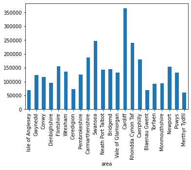
Bar chart¶

# use area names column as index (instead of row numbers) - this will label the x axis

pop.set_index('area', inplace=True)

pop.head()

	pop_one	pop_eighteen
area
Isle of Anglesey	67806	69961
Gwynedd	116844	124178
Conwy	109674	117181
Denbighshire	93070	95330
Flintshire	148629	155593

# bar chart

pop.pop_eighteen.plot(kind = 'bar')

# this works a placeholder 'do nothing' but here stops the <AxesSubplot:title ETC. A semicolon also works
pass

_images/viz_pandas_syntax_12_0.png

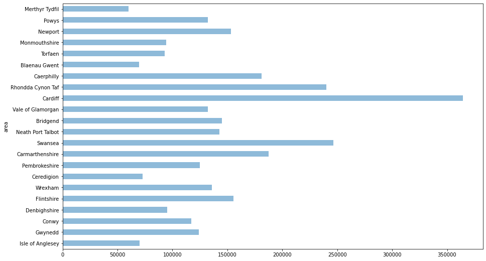
# # horizontal bar chart, with adjusted opacity, title and figure size

pop.pop_eighteen.plot(kind = 'barh', alpha = 0.5, figsize=(15,9));

_images/viz_pandas_syntax_14_0.png

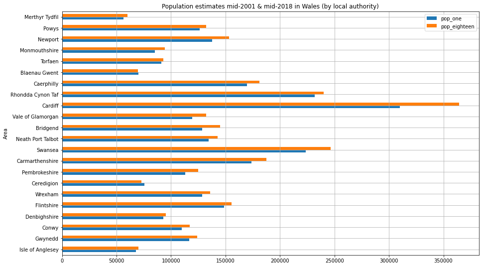
# stacked barchart with title, grid and labels

pop[['pop_one','pop_eighteen']].plot(kind = 'barh', 
                                     figsize=(15,9),
                                     title = 'Population estimates mid-2001 & mid-2018 in Wales (by local authority)',
                                     grid = True,
                                     stacked = False,
                                     xlabel = 'Area', 
                                     ylabel = 'Population');

_images/viz_pandas_syntax_15_0.png

Linechart¶

using numbers of pubs in Wales by local authority 2001-18

path = '/Users/aidanair/Documents/DATA/ALL_DATASETS/'
file = 'wales_pubs_area_2001_18.csv'

# give the df a variable name 'years'
years = pd.read_csv(path + file)

years[:2]

	code	area	2001	2002	2003	2004	2005	2006	2007	2008	2009	2010	2011	2012	2013	2014	2015	2016	2017	2018
0	W06000001	Isle of Anglesey	75	85	90	85	85	90	90	80	80	75	70	75	55	60	60	60	60	60
1	W06000002	Gwynedd	135	135	145	145	135	145	150	160	150	135	130	140	140	140	125	120	120	120

# delete the 'code' column

del years['code']

# set the area name as the index

years = years.set_index('area')

years[:2]

	2001	2002	2003	2004	2005	2006	2007	2008	2009	2010	2011	2012	2013	2014	2015	2016	2017	2018
area
Isle of Anglesey	75	85	90	85	85	90	90	80	80	75	70	75	55	60	60	60	60	60
Gwynedd	135	135	145	145	135	145	150	160	150	135	130	140	140	140	125	120	120	120

# transpose to set the years as the y axis and rename the vertical axis as 'year'

years = years.transpose().rename_axis('year', axis=1)

years[:2]

year	Isle of Anglesey	Gwynedd	Conwy	Denbighshire	Flintshire	Wrexham	Ceredigion	Pembrokeshire	Carmarthenshire	Swansea	...	Vale of Glamorgan	Cardiff	Rhondda Cynon Taf	Caerphilly	Blaenau Gwent	Torfaen	Monmouthshire	Newport	Powys	Merthyr Tydfil
2001	75	135	105	110	145	130	75	205	225	200	...	100	220	185	130	45	75	115	105	235	55
2002	85	135	115	120	145	140	80	205	235	230	...	100	240	195	140	55	85	125	105	230	55

2 rows × 22 columns

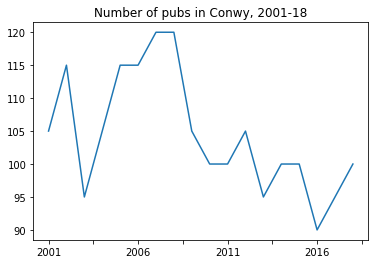
# plot a single column by time

years.Conwy.plot(title = 'Number of pubs in Conwy, 2001-18');

_images/viz_pandas_syntax_24_0.png

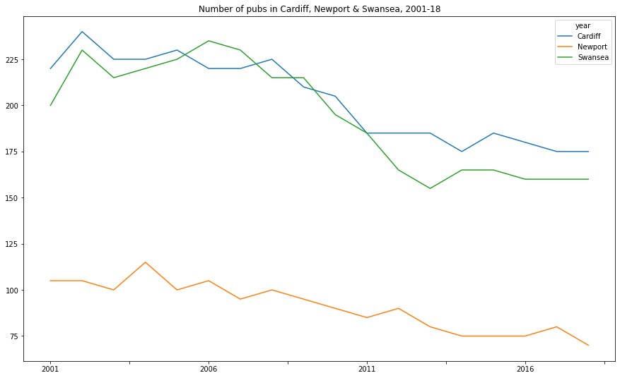
# plot a selection of columns

years[['Cardiff', 'Newport', 'Swansea']].plot(figsize = (15, 9), title = 'Number of pubs in Cardiff, Newport & Swansea, 2001-18');

_images/viz_pandas_syntax_25_0.png

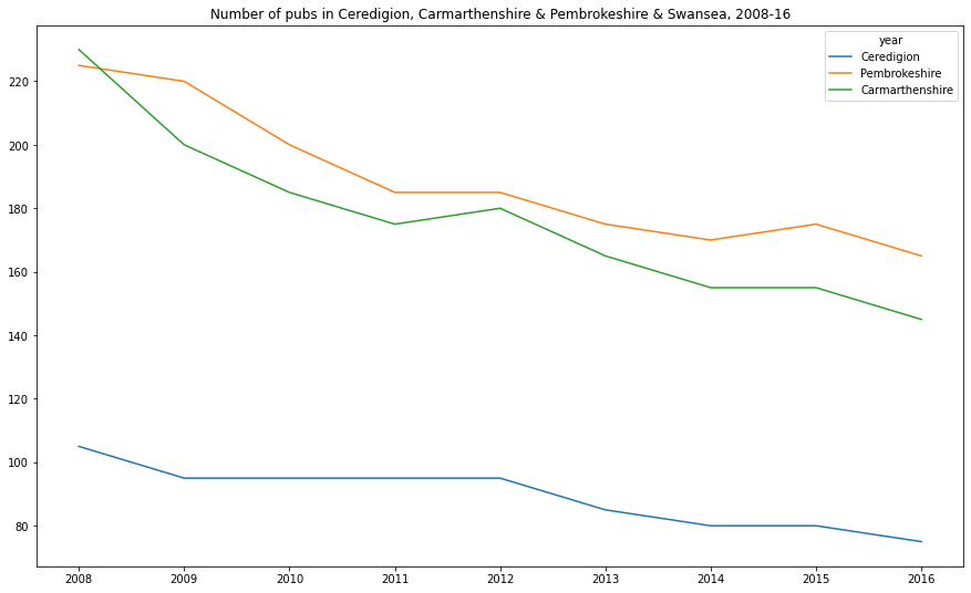
# plot a period and several areas

years['2008':'2016'][['Ceredigion', 'Pembrokeshire', 'Carmarthenshire']].plot(figsize = (15, 9), 
                                                                             title = 'Number of pubs in Ceredigion, Carmarthenshire & Pembrokeshire & Swansea, 2008-16');

_images/viz_pandas_syntax_26_0.png

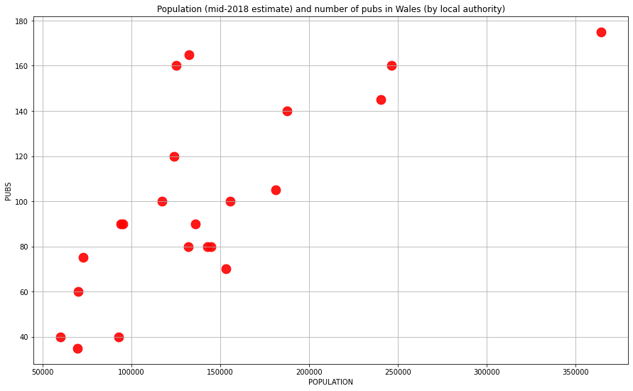
Scatterplot¶

Wales pubs and population in 2018: gives a (dependent) variable to set against population: the number of pubs in local authorities

path = '/Users/aidanair/Documents/DATA/ALL_DATASETS/'
file = 'wales_all.csv'

pp = pd.read_csv(path + file)

pp[:3]

	area	pubs	pop
0	Isle of Anglesey	60	69961
1	Gwynedd	120	124178
2	Conwy	100	117181

# scatterplot with dotsize (s) and dotcolour (c)

pp.plot(kind = 'scatter', 
        x = 'pop', 
        y = 'pubs', 
        figsize=(15,9),
        alpha = 0.9,
        title = ('Population (mid-2018 estimate) and number of pubs in Wales (by local authority)'),
        grid = True,
        s = 165, 
        c = 'r',
        xlabel = 'POPULATION',
        ylabel = 'PUBS')

# save to current directory
plt.savefig('wales_pop_pub.png')

_images/viz_pandas_syntax_30_0.png

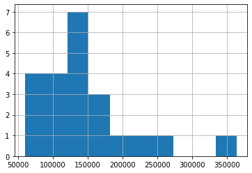
Histogram¶

# histogram on a single column

pop.pop_eighteen.hist();

_images/viz_pandas_syntax_32_0.png

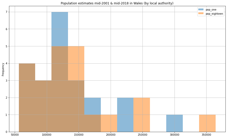
# histogram on both cols

pop[['pop_one','pop_eighteen']].plot(kind = 'hist', 
                                     alpha = 0.5, 
                                     figsize=(15,9),
                                     title = 'Population estimates mid-2001 & mid-2018 in Wales (by local authority)',
                                     grid = True,
                                     stacked = False,
                                     bins = 12,
                                     xlabel = 'Area', 
                                     ylabel = 'Population');

_images/viz_pandas_syntax_33_0.png

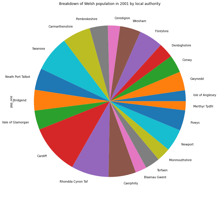
Piechart¶

# piechart

pop['pop_one'].plot.pie(figsize=(20,12), title = 'Breakdown of Welsh population in 2001 by local authority');

_images/viz_pandas_syntax_35_0.png

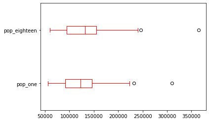
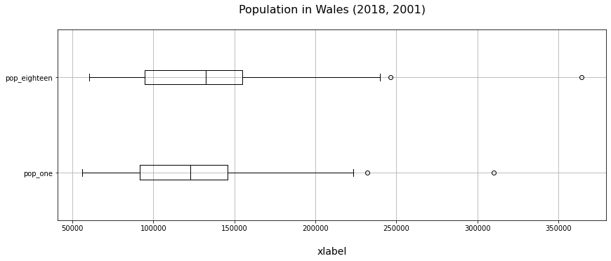
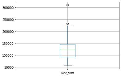
Boxplot¶

plt.figure(figsize=(14, 5))

pop.boxplot(vert=False, color = 'black')

plt.xlabel('\nxlabel', fontsize = 14)
# plt.legend(topleft)

plt.title('Population in Wales (2018, 2001)\n', fontsize = 16)

plt.show()

_images/viz_pandas_syntax_37_0.png

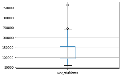
# box plots by single column...

pop.boxplot('pop_one'); 

_images/viz_pandas_syntax_38_0.png

pop.boxplot('pop_eighteen');

_images/viz_pandas_syntax_39_0.png

# ... and by df (with default vertical turned off) and colour selected

pop.boxplot(vert = False, grid = False, color = 'red');

_images/viz_pandas_syntax_40_0.png

14,000 Bees Summary statistics