WALKTHROUGH: Calculations in a spreadsheet
Often, the fastest way to interview a dataset (“Who had the most…?”, “Which company changed the least…?” etc.) is to use simple calculations or functions that are built into your spreadsheet programme. These take the information in cells and calculate, for example, the maximum value or the average value or the sum of all the values and so on.
PREPARATION
Taking the plastic bags dataset you’ve already used, filter for just the year 2019-20 then copy the column names and all cells with information and paste them into a new sheet.
Give the sheet a name (on the tab in the bottom left), rename the columns, freeze the top row (under the View tab) and sort (Z-A) by the number-of-bags column so the biggest numbers are at the top.
Your sheet has the number of bags and the proceeds for all 194 retail companies in the year 2019-20.
CALCULATING
Type this into any available empty cell and hit Enter.
=C2+C3+C4
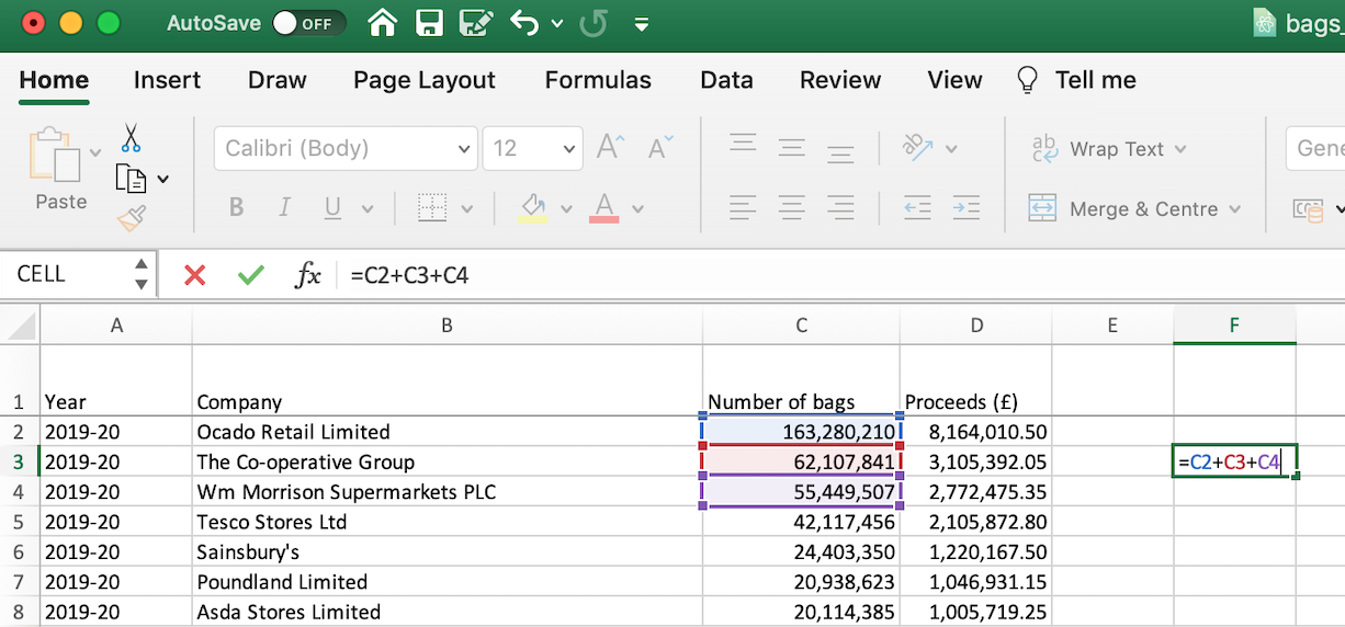
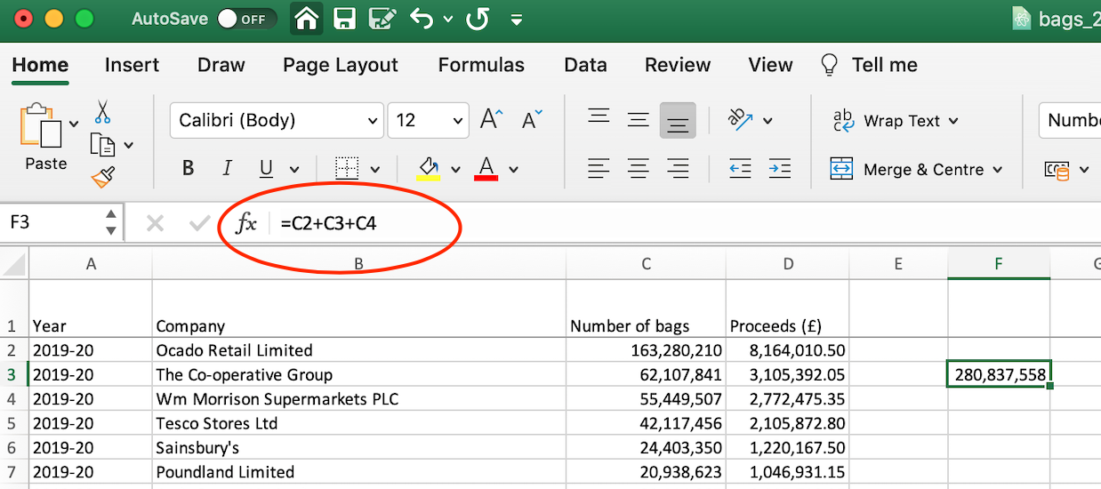
It will give you the sum of the cells C2, C3 and C4, which is the total number of bags in 2019-20 from the top three retailer chains (by numbers of bags)
When you select the cell (which shows around 280 million), you can see the calculation (=C2+C3+C4) in the upper left of the sheet:
=D2/C2
is a simple calculation to divide one cell by another. Here, it will divide the money taken in by Ocado (D2) by the number of bags given out by Ocado (C2) and show you how much was paid per bag by customers.
=SUM(C2:C11)
will give you the total number of bags for the top ten retailer chains: all the cells from C2 to C11
=SUM(C2:C195)
will add all the numbers in Column C and give you the total number of bags distributed by the retailers
=AVERAGE(C2:C195)
will give you the average number of bags handed out by a retail chain that year
=SUM(C2:C195) / 52
takes the total number of bags for England in 2019-20 and divides by 52 for an overall weekly average
=COUNTA(B2:B195)
‘Count A’ will count all items in a column (not just numbers). Here it returns 194 for the number of retailers in Column B
=COUNTIF(B2:B195, “*university*”)
‘Count if’ will count a cell only if it meets a criterion. Here the cell needs to contain the word ‘university’ if it’s to be counted (the * is a wildcard and means anything can appear right before or right after the word).
You can also just use CMD / CTRL + F to Find the word and count each occurrence (here there are only six instances of the word).